With Superbowl 50 this weekend, we thought it would be fun to use Python to look back at last year’s Superbowl between the Seattle Seahawks and New England Patriots and demonstrate how to create NFL drive charts in ArcGIS. A drive chart is a visual representation of a sequence of plays during a football game. Here, we’ll show how you can use Python and ArcGIS to summarize all of the drives from Superbowl XLIX and also how you can display the plays from individual drives.
For this post we used the following imports:
import os
import nflgame
import arcpy
The nflgame package is an API that is used to read and retrieve NFL Game Center JSON data. It is a convenient package for accessing NFL statistics for multiple games, parsing data for individual games, and working with real-time game data.
The Football Field
The first thing we did was create the football field. We created a football field feature class, assembled polygon features for the field, and inserted them into the feature class with an insert cursor. Here is our function to create the football field:
def build_football_field(output_gdb, output_feature_class):
    print('Creating football field.')
    footbal_field_fields = ('SHAPE@', 'TEAM')
    fc = os.path.join(output_gdb, output_feature_class)
    if not arcpy.Exists(os.path.join(output_gdb, output_feature_class)):
        arcpy.CreateFeatureclass_management(
            output_gdb, output_feature_class, "POLYGON", "#", "DISABLED",
            "DISABLED", arcpy.SpatialReference(3857))
        arcpy.AddField_management(fc, footbal_field_fields[1], "TEXT",
                                  field_length=20)

    cursor = arcpy.da.InsertCursor(fc, footbal_field_fields)

    field = [(0, 533.3),
             (1000, 533.3),
             (1000, 0),
             (0, 0)]
    cursor.insertRow([field, ""])

    home_endzone = [(-100, 533.3),
                    (0, 533.3),
                    (0, 0),
                    (-100, 0)]
    cursor.insertRow([home_endzone, "SEATTLE"])

    away_endzone = [(1000, 533.3),
                    (1100, 533.3),
                    (1100, 0),
                    (1000, 0)]
    cursor.insertRow([away_endzone, "NEW ENGLAND"])
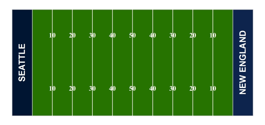
The dimensions of a football field are 100 yards x 53.33 yards with endzones that are 10 yards deep. We scaled the length and width up by a factor or 10. We also created the yardline markers spaced at 10 yard intervals. The ‘MARKER’ field was used to label the yardlines. Here is our function to create the yardlines:
def build_yard_lines(output_gdb, output_feature_class):
    print('Creating yard markers.')
    footbal_line_fields = ('SHAPE@', 'MARKER')
    fc = os.path.join(output_gdb, output_feature_class)
    if not arcpy.Exists(os.path.join(output_gdb, output_feature_class)):
        arcpy.CreateFeatureclass_management(
            output_gdb, output_feature_class, "POLYLINE", "#", "DISABLED",
            "DISABLED", arcpy.SpatialReference(3857))
        arcpy.AddField_management(fc, footbal_line_fields[1], "TEXT",
                                  field_length=10)

    cursor = arcpy.da.InsertCursor(fc, footbal_line_fields)
    markers = [10, 20, 30, 40, 50, 60, 70, 80, 90]
    for marker in markers:
        line_1 = [(marker * 10, 533.3 / 2), (marker * 10, 0)]
        line_2 = [(marker * 10, 533.3 / 2), (marker * 10, 533.3)]
        if marker > 50:
            cursor.insertRow([line_1, str(100 - marker)])
            cursor.insertRow([line_2, str(100 - marker)])
        else:
            cursor.insertRow([line_1, str(marker)])
            cursor.insertRow([line_2, str(marker)])
After creating the field and yardline features, we brought them into ArcMap and designed the field. Here’s what it looks like:
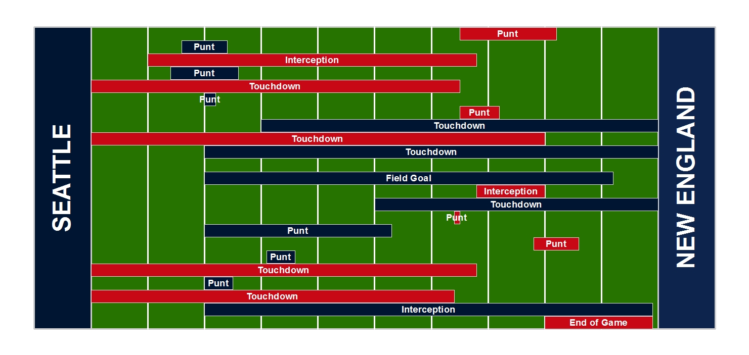
The Drive Chart
Next, we created a drive chart showing the results of every drive from Superbowl XLIX. We used nflgame to access the drive data, arcpy to create a drive chart feature class, and an insert cursor to add the geometries and attribution to the feature class. In order to get all of the drive and play data, we created a game object for a single game, i.e. Superbowl XLIX. From the game object, we retrieved a list of all of the drives. Here’s the code:
home = 'SEA'      #Seattle Seahawks
away = 'NE'       #New England Patriots
year = 2014       #2014 Season
week = 5          #Week 5
reg_post = 'POST' #Postseason

print('Getting game data.')
game = nflgame.one(year, week, home, away, reg_post)

print('Getting drive data.')
drives = get_game_drives(game)
drive_count = get_num_drives(drives)
where get_game_drives returns a list of drives
def get_game_drives(game):
    return [drive for drive in game.drives]
and get_num_drives returns the number of drives per game.
def get_num_drives(drives):
    for drive in drives:
        drive_count = drive.drive_num

    return drive_count
We created a feature class to insert the drive data into. This feature class contained the following fields:
drive_fields = ('SHAPE@', 'TEAM', 'DRIVE_NUM', 'START_POS', 'END_POS',
                'DURATION', 'RESULT', 'DESCRIPTION')
where,
- ‘SHAPE@’ is the shape of the bar representing the drive
- ‘TEAM’ is the team that had possession of the football
- ‘DRIVE_NUM’ is the number of the drive
- ‘START_POS’ is the yardline where the drive started
- ‘END_POS’ is the yardline where the drive ended
- ‘DURATION’ is the length of time the drive took
- ‘RESULT’ is the outcome of the drive
- ‘DESCRIPTION’ is the NFL Game Center description of the drive
Then, we opened up an insert cursor for the drive chart feature class, and for every drive in the drives object, we created a drive chart polygon and populated the above attribute fields.
print('Opening insert cursor.')
cursor = arcpy.da.InsertCursor(os.path.join(output_gdb, output_fc),
                               drive_fields)

drive_bar_height = 533.3 / drive_count
for drive in drives:
    if drive.field_start:
        start_x, end_x = create_chart_polygon(drive, home, away)
        if start_x == end_x:
            polygon = [
                (start_x, (drive_count - drive.drive_num) * drive_bar_height),
                (end_x + 0.1, (drive_count - drive.drive_num) * drive_bar_height),
                (end_x + 0.1, (drive_count - drive.drive_num) * drive_bar_height + (drive_bar_height - 1)),
                (start_x, (drive_count - drive.drive_num) * drive_bar_height + (drive_bar_height - 1))]
        else:
            polygon = [
                (start_x, (drive_count - drive.drive_num) * drive_bar_height),
                (end_x, (drive_count - drive.drive_num) * drive_bar_height),
                (end_x, (drive_count - drive.drive_num) * drive_bar_height + (drive_bar_height - 1)),
                (start_x, (drive_count - drive.drive_num) * drive_bar_height + (drive_bar_height - 1))]

        cursor.insertRow([polygon, drive.team, drive.drive_num,
                          str(drive.field_start), str(drive.field_end),
                          str(drive.pos_time.__dict__['minutes']) + ' min and ' +
                          str(drive.pos_time.__dict__['seconds']) + ' sec',
                          drive.result, str(drive)])
Here, create_chart_polygon returns the start position (start_x) and end position (end_x) for each drive and looks like:
def create_chart_polygon(drive, home, away):
    scale_by = 10
    if drive.team == home:
        start_x = 50 + drive.field_start.__dict__['offset']
        if drive.result == 'Touchdown':
            end_x = 100
        else:
            end_x = 50 + drive.field_end.__dict__['offset']

    if drive.team == away:
        start_x = 50 - drive.field_start.__dict__['offset']
        if drive.result == 'Touchdown':
            end_x = 0
        else:
            end_x = 50 - drive.field_end.__dict__['offset']

    return scale_by * start_x, scale_by * end_x
After creating the drive chart, we added it to the football field above, symbolized the drives by the ‘TEAM’ field (Seattle is dark blue, New England is red), and added labels corresponding to the ‘RESULT’ field. Here’s what the drive chart looks like.
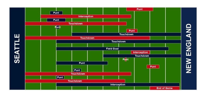
Drives are ordered from top to bottom, with the top of the chart being the first drive of the game and the bottom being the last.
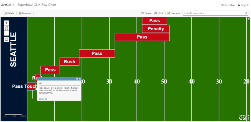
Individual Drives
We also mapped individual drives. This allows us to look at the plays within the drive and understand how the team moved down the field. If you’re interested in all the details, you can check out our sourcecode on Github. In a nutshell, for every drive we returned the plays and following from the same logic above for the drive chart, we created polygons for each play within the drive. In this case, we created a feature class for every drive and populated the following attribute fields:
play_fields = ('SHAPE@', 'TEAM', 'DRIVE_NUM', 'START_POS', 'END_POS',
               'DURATION', 'PLAY', 'RESULT', 'DESCRIPTION')
The field names are the same as for the drives, except we added a ‘PLAY’ field that indicates the type of play, for example, a “rush”, “pass”, “kick”, etc.
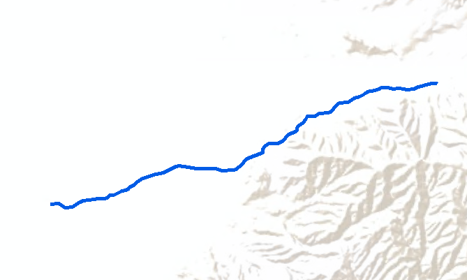
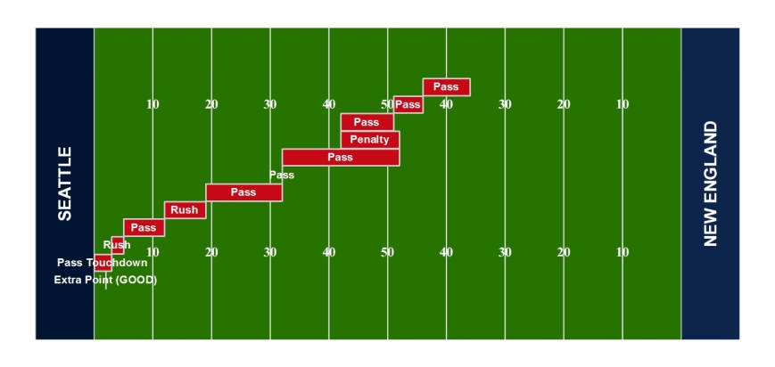
The New England Patriots won Superbowl XLIX 28-24 and on their second to last drive, they took the lead on a touchdown pass from Tom Brady to Julian Edelman. Here’s the play chart.
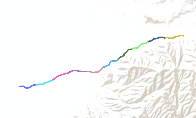
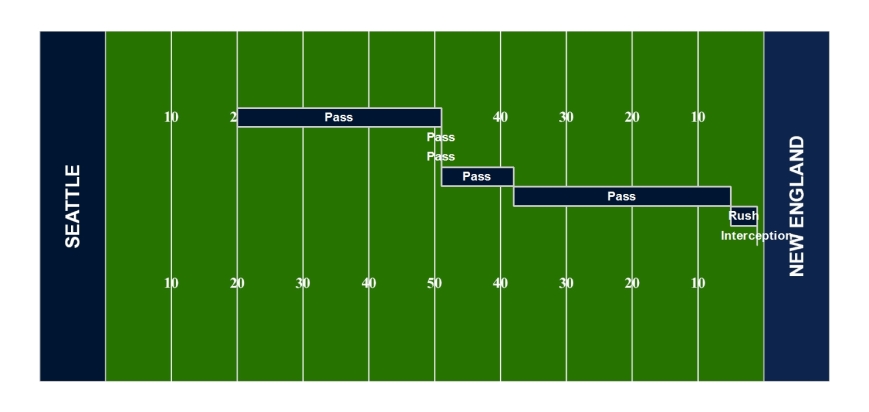
On the following drive, the Seattle Seahawks had a chance to win the game, but Malcolm Butler intercepted a pass from Russell Wilson to seal the game for the Patriots.
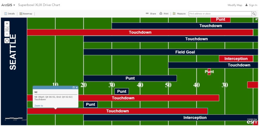
Drives as Webmaps
We shared the drive charts as webmaps. This allows you to interact with the charts and design popups to view the play results and other attributes. Click on each image to go to the webmap.
Feel free to leave any comments or questions in the comment box.
Happy coding,
-the arcpy team